Many of the figures that I produce are based on elaborations of Lissajous Curves. Like many physicists and engineers of my generation I first encountered these when using electronic oscilloscopes in laboratories. These are often used for displaying electronic wave forms against time. In those days we used cathode ray tubes and an electron beam was swept from left to right at regular high speed, while the waveform voltage was applied in such a way that it deflected the beam up or down according to the instantaneous voltage. So, by playing a pure tone from a signal generator into the oscilloscope we could trace a sine wave on the screen.
 |
 |
 |
 |
 |
 |
Most oscilloscopes also allowed you to control the horizontal sweeping of the beam with an applied voltage, which might perhaps be from a second signal generator playing a different frequency. Interesting curves were produced when the ratios of the two frequencies has a simple relationship. Lissajous himself lived before the time of electronics, but he attached mirrors to the arms of tuning forks held at right angles to each other, and projects a bright beam of light from one mirror to the other to trace curves with the light. Later, people made mechanical devices with multiple pendulums, called harmonographs. One pendulum might control the movement of a pen from side to side, while a second pendulum moved it up and down. A simple Lissajous curve in itself soon gets visually boring, but the nature of mechanical pendulums which are subject to friction inevitably implies decaying amplitudes so figures traced gradually reduced in size and the overlapping lines increased the visual appeal.
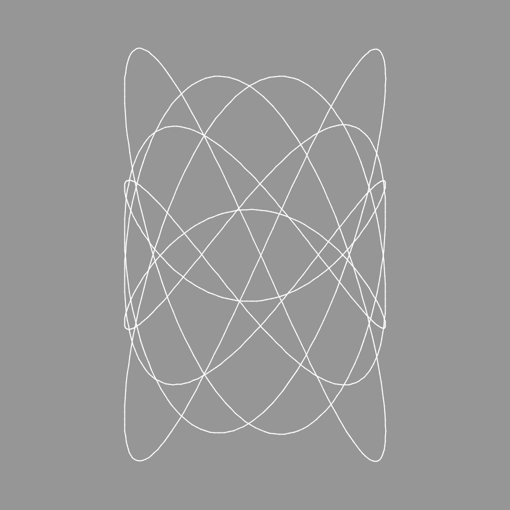
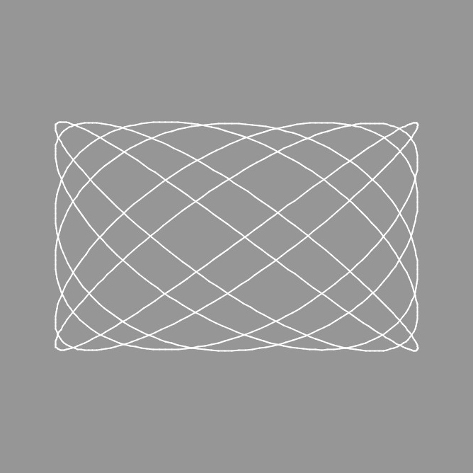
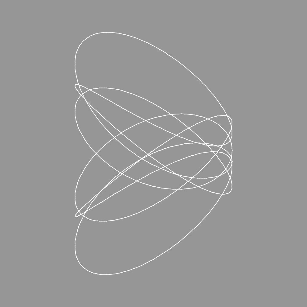
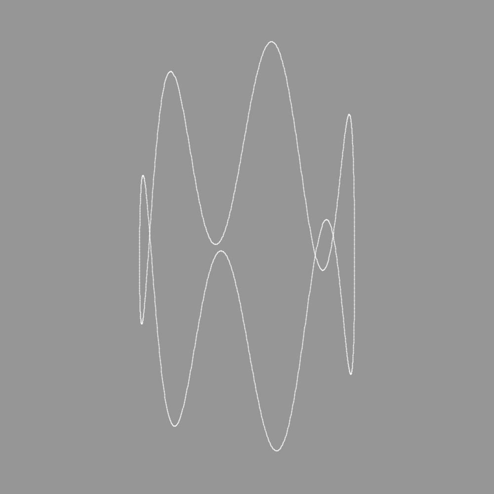
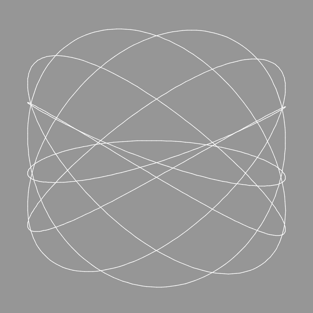
It is much easier in Processing. We just define an x-coordinate using an expressions like x[i] = Ax sin(n*t[i] + px) and a corresponding y-coordinate with y[i] = Ay sin(m*t[i] + py), where t[i] is a regularly increasing value of time. Then we draw the lines from the point x[0],y[0] to x[1],y[1], followed by x[1],y[1] to x[2],y[2] and so on. In computing jargon this is iterating over the values i and time, t[i]. If we wish, we can also arrange for the amplitude of the oscillations to decay over time, just like a physical pendulum in a harmonograph.
We can play with the values of n and m (which determine the frequency with which x and y coordinates oscillate backwards and forwards), px, and py (which are phases - a technical term which essentially means time delays measuring in fractions of the oscillation period) and the amplitudes Ax and Ay. A Processing sketch that traces simple Lissajous curves can be found here. (Paste it into a Processing Sketch.) Some examples produced with this program are shown above.
Rather than tracing the Lissajous curve itself as illustrated above we can instead choose to draw a motive at each iteration point we touch while drawing the curve. Our motif might just be a straight line at some angle that is itself allowed to rotate. The combination of such lines based on the curve tends to generate caustic curves. See the Lissajous Curve Gallery or a few example below. Some of these simulate the decay effect of harmonograph pendulums.
As always with Processing, it is relatively straightforward to elaborate the basic idea to a point so far beyond earlier conceptions that at first sight it seems to have little relationship with its origins. The "Waves" series of productions in the Generative Art Gallery are based around elaborations of a simple Lissajous curve using variations on a wave motif.
The following example programs can be downloaded via the hyperlinks to produce basic images (illustrated in the thumbnail) from which you can experiment further. (Click on the thumbnail to see higher resolution images. Some of the subtleties in these images is in the fine-grained textures so the thumbnails do not adequately represent the full image.)
In each case the hyperlinked example program text will usually produce the image displayed on the right more or less exactly. However, the Galleries usually contain a series of similar images from the same variant of the program using different configuration parameters.
| Basic Lissajous Curve Generator: This interactively allows different curves to be explored. | |
| Lissajous 1: Follow a simple Lissajous curve where an elliptical motif is drawn at each iteration of draw(). Experiments with this program, besides changing the various oscillation periods might involve changing the ellipse motif to a line (but remember to also increase the opacity of lines (using the parameter in the stroke() subroutine) otherwise they will hardly be visible. | |
| Lissajous 2: This time the basic motif is a three lines radiating from the point being traced on the curve. The program has also been improved by moving the configuration parameters to a group defined in the global area, rather than leaving them as numbers written "in-line" in the draw() subroutine. | |
| Lissajous 3: Another example using a single line and a simple decaying epicycle (which is a constrained variation on a Lissajous curve. This time the x,y coordinates are determined by subroutines, and the motif uses some basic trigonometry to make a perpendicular line the the curve. | |
| Waves 1: This somewhat gaudy result is the effect of drawing a a wave motif out from a Lissajous curve. Increase the rotation rate of the motif - say dth=0.007 and put rotate(7*dth*t) instead of rotate(t*dth) use a small wave amplitude, amp, to obtain strikingly different results. | |
| Waves 6: Is rather similar to Waves 1, but with slightly different oscillation parameters. In addition the first few wave lines fade in gradually rather that at full strength. This makes it less obvious where the figure started (no "hard edge" for the first motif drawn). | |
| Waves 8: A minor developments of the Waves 6 program. Firstly the wavy-line motif is allowed to fade as the line moves away from the center of the screen. Secondly, if the user presses and releases the "o" key, the entire motif fades to invisibility, removing all suggestions of a sharp finish to the production. Other program parameters have also been adjusted to get a different evolution of the image from the same algorithm. | |
|
Waves 9: The program is essentially the same as Waves 8, except that all the configurable parameters are now declared as global variables. This is part of the process of re-organising what has already been done to make the operation of the program more transparent prior to adding new features. It is very rarely the case that one gets the best program design at the first attempt. Time spent improving what you have already done is almost never wasted when you wish to take the development further. Once again, the oscillation parameters of the algorithm have been changed to give a different outcome. |
|
|
Waves 10: The wavy line motif is now drawn in a subroutine, and no longer has a quite such a regular waveform. This will facilitate the a future stage of development where the line may be allowed to develop random variations in shape. Such an increase in complexity would be difficult to follow and get right if we did not simplify before more complexity. Once again, of course, we play with the algorithms parameters to get a different production. |
|
|
Waves 11: The program is becoming increasingly complex as I add more features. The overall size of the Lissajous curve and the opacity now decrease exponentially with time (simulating the decay of a harmonograph). We also let the opacity of the wave motif vary with time, and instead of only saving an image when the user presses the "s" key we now do an automatic save at predefined intervals, so one can walk away from the computer and let a series of images build up. (It is normally the case that the most pleasing images are not the last ones to be created. In most of the images produced with this variant of the program it seems to take about 20,000 iterations of draw() - perhaps 10 to 15 minutes of computing time - to produce a satisfying image - but it often begins to looks overworked by 25,000 iterations.) In order to control this increasing complexity, before going on a do some re-organisation in order to make the algorithm easier to follow. (There is no fundamental change in what it does, but it is easier to see what it is supposed to be doing.) This will help as we move to a more complex algorithm. It is NEVER the right choice simply to go on adding new features without re-considering the design of what you already have. I ALWAYS ask "Had I known where I have ended up now, would I have designed the program like this?" The answer is normally "No!" and experience assures me that the future development will continue at a faster pace if I re-organise and simplify before proceeding further. |
|
|
Waves 12: This may be the last version of the this line of exploration for a while. I feel it is time to move in a different direction and learn some new techniques. I hope, however, to leave things where I have been aiming since I started this series, by introducing a certain amount of randomness into the image generation. This Gallery shows some of the results, which to my taste have more pleasing textures that the previous experiments. This is achieved by introducing small random variations into the component harmonics from which the wave motif is constructed (this means that the motif has to be rebuilt each time it is drawn, taking a little more computing time). By introducing the variation in this way we retain the overall smoothness of the wave motif and avoid any large changes from the previous time it was drawn. Colour is also allowed to vary slightly each time, nudging the RGB values up or down usually by one unit. This is difficult for the eye to distinguish in adjacent traces, but over, say, 20,000 iterations (which is typical in these trials) the colour makes a random walk in RGB space that eventually takes it a long way from the starting point (and in a different direction each time the program is executed). The image on the right was generated from the linked version of the program - this is where I ended up. It is not, perhaps, the most interesting of this series, but you are free to play with the configuration parameters, remembering that the use of random number means that no two executions will produce identical results. |
|
|
Waves 13: I could not leave this idea alone just yet - though the only reason it should be discussed on the "Lissajous Curves" page is that it is a development of the same theme. However, instead of using an underlying Lissajous curve to trace a path on the image, above which the wave motif is drawn, I wondered what would happen if I introduced some randomness into the curve itself. See the "Waves 13" Gallery for some results and my Complex Dynamics page for more discussion. I did consider randomly adjusting the parameters controlling the Lissajous Curve while it was being drawn, but it seemed to be even more interesting to take a larger step towards a completely chaotic curve, generated using a physical problem known to have complex dynamics, that is, the curve is completely deterministic - like Lissajous curve - but guaranteed to be non-periodic and exhibits behaviour that looks highly random if you do not understand the underlying process. The weather is another example of a big system with complex dynamics. However, this really is too complicated for our purposes, so I chose to simulate the movement of a small space satellite moving under the influence of two gravitational attractors (e.g. planets). This is in principle a very simple problem (at least to describe). It is a bit harder to simulate (certainly compared to programming a Lissajous curve) but still only requiring one smallish subroutine in the program. |
