Lissajous Curves

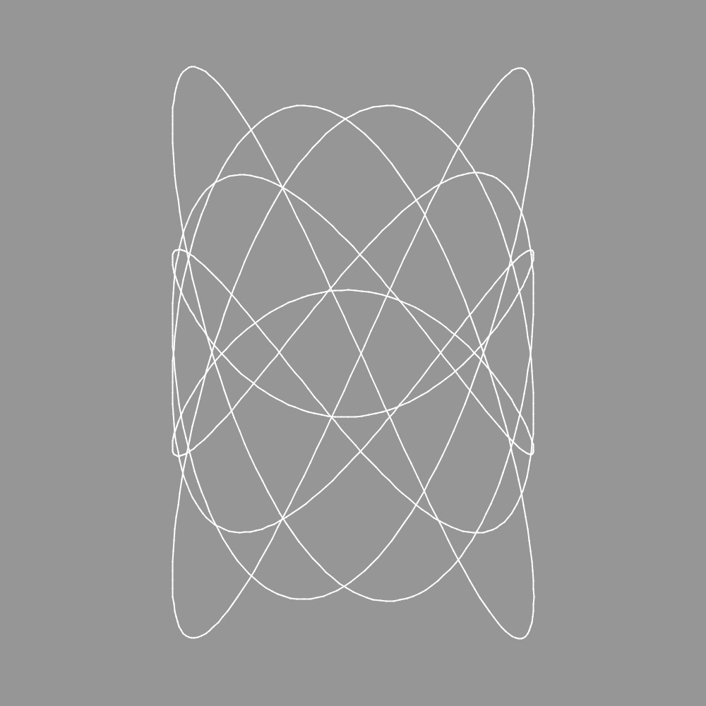
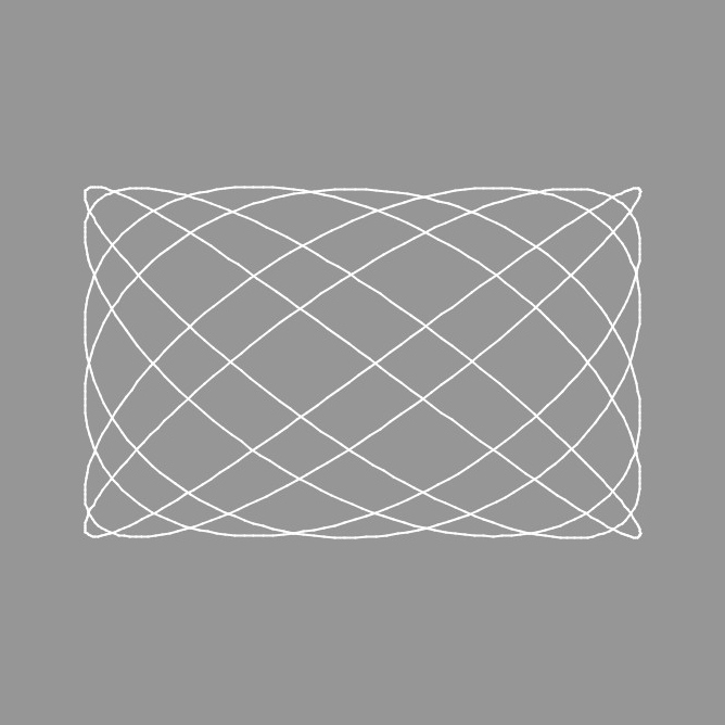
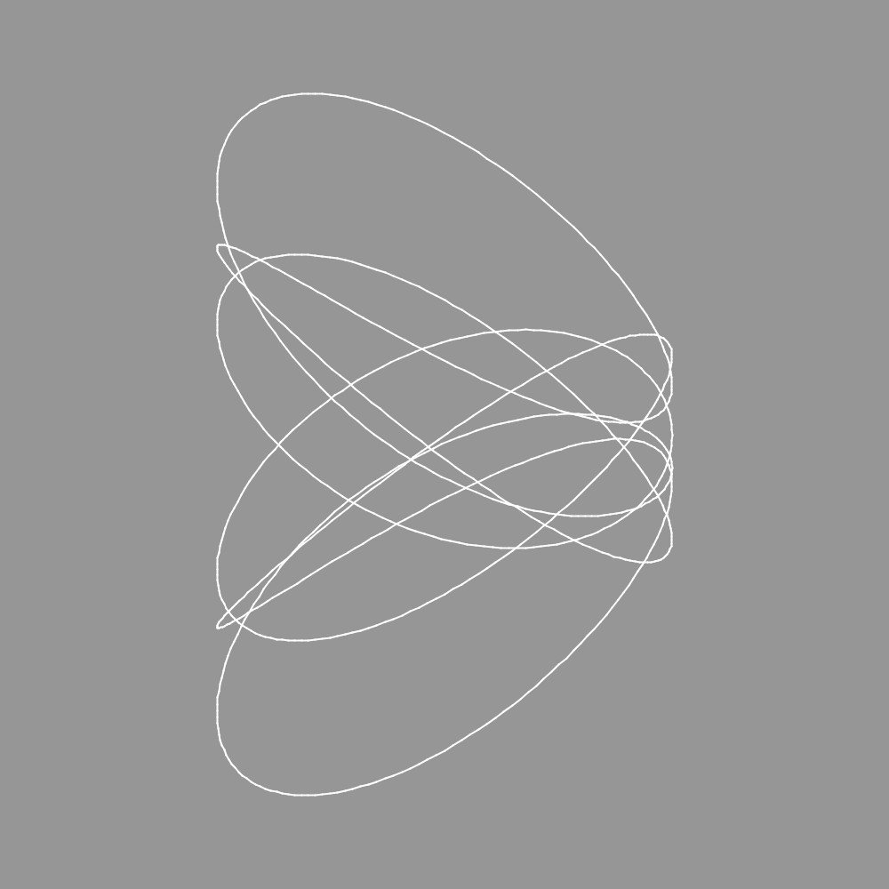
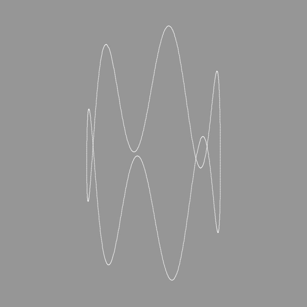
Many of the figures that I produce are based on elaborations of Lissajous Curves. Like many physicists and engineers of my generation I first encountered these when using electronic oscilloscopes in laboratories. These are often used for displaying electronic wave forms against time. In those days we used cathode ray tubes and an electron beam was swept from left to right at regular high speed, while the waveform voltage was applied in such a way that it deflected the beam up or down according to the instantaneous voltage. So, by playing a pure tone from a signal generator into the oscilloscope we could trace a sine wave on the screen. 

Most oscilloscopes also allowed you to control the horizontal sweeping of the beam with an applied voltage, which might perhaps be from a second signal generator playing a different frequency. Interesting curves were produced when the ratios of the two frequencies has a simple relationship. Lissajous himself lived before the time of electronics, but he attached mirrors to the arms of tuning forks held at right angles to each other, and projects a bright beam of light from one mirror to the other to trace curves with the light. Later, people made mechanical devices with multiple pendulums, called harmonographs. One pendulum might control the movement of a pen from side to side, while a second pendulum moved it up and down. A simple Lissajous curve in itself soon gets visually boring, but the nature of mechanical pendulums which are subject to friction inevitably implies decaying amplitudes so figures traced gradually reduced in size and the overlapping lines increased the visual appeal.

It is much easier in Processing. We just define an x-coordinate using an expressions like x[i] = A_x sin(n*t[i] + p_x)  and a corresponding y-coordinate with y[i] = A_y sin(m*t[i] + p_y), where t[i] is a regularly increasing value of time. Then we draw the lines from the point x[0],y[0] to x[1],y[1], followed by x[1],y[1] to x[2],y[2] and so on. In computing jargon this is iterating over the values i and time, t[i]. If we wish, we can also arrange for the amplitude of the oscillations to decay over time, just like a physical pendulum in a harmonograph.

We can play with the values of n and m (which determine the frequency with which x and y coordinates oscillate backwards and forwards), p_x, and p_y (which are phases - a technical term which essentially means time delays measuring in fractions of the oscillation period) and the amplitudes A_x and A_y. A Processing sketch that traces simple Lissajous curves can be found here. (Paste it into a Processing Sketch.) Some examples produced with this program are shown above.